Engineers at Work: Enhancing Aperture with Elasticsearch and MongoDB
Nov 16, 2017
8 minutes
21 views

Aperture is our enterprise security SaaS tool that collects data from the cloud to build a threat prevention model for administrators of cloud-based collaboration applications (Box, Dropbox, Google Drive, Microsoft Office, etc.). Once this model is constructed, we can take multiple steps to mitigate various risks by either quarantining files or reducing their sharing permissions.
One of the most useful aspects of Aperture is the ability to slice and dice data in various ways on all aspects of the threat model. For example, we provide access permission information on individual files based on public links, and then we go further to provide a high-level view of how many objects are exposed either to anonymous users or specific non-company users. We provide this view in near-real time with respect to when we receive data.
In other words, as soon as Aperture becomes aware of the presence of a new public link, we can provide this information with a roll-up of statistics, such as files with public links and potential sensitive information, or source code files with public links. In addition, we provide a way for customers to filter activity-based information on users, event types (download, upload, etc.), chronology and other facets. This is also done in near-real time to provide fast access to activity-based data for our customers to sift through.
Aperture uses MongoDB to store a lot of the persistent information related to these collaboration applications. MongoDB is a perfectly functional database for storing unstructured data in a JSON format while accessing this data using _id or indexing a subset of the fields used in frequent queries.
However, we realized we needed a better tool when querying millions of documents while filtering and aggregating across more than 15 columns, especially as these queries would be concurrent for each user and ingesting tens of thousands of documents per second. In this blog, we’ll share how we strategically maximize our use of MongoDB.
Keeping Data in Sync Between Both Databases
Choosing a Database
When attempting to decide between various databases that would fit our needs, we shortlisted Elasticsearch, Solr, and Postgres, and listed pros and cons for each.
| Database | Pros | Cons |
| Elasticsearch |
|
|
| Postgres or similar SQL |
|
|
| Solr |
|
|
We selected Elasticsearch for the simple reason that it comes with built-in sharding, which allows us to scale the nodes on demand. The issue of data not being reliably persistent was acceptable as we planned to copy the data from MongoDB, our persistent datastore.
First Attempt: Elasticsearch + MongoDB River
The first version of our Elasticsearch-based engine used MongoDB River to ingest data from MongoDB to be indexed in Elasticsearch.
Elasticsearch, at the time, supported Rivers, which would essentially run on the Elasticsearch cluster and automatically ingest data from any other location.
The MongoDB River was a plugin built by the community and installed at the time of Elasticsearch deployment. After “starting” the plugin with the MongoDB username and password, there was a two-step process to bring the Elasticsearch index in line with the Mongo collection:
- Record the oplog timestamp, then use a cursor to iterate through the list of documents and ingest them.
- Tail the oplog from the recorded timestamp and update data in the index accordingly.
This worked fine until we reached a critical mass in terms of writes (updates and deletes). When the workload got too heavy, the index ingestion would take longer than MongoDB's available oplog data. This meant the index would be out of date before it had even ingested the entire collection. Heavy write load across multiple MongoDB clusters loaded our Elasticsearch cluster to the point that indices would require regular rebuilding. Elasticsearch “cpu-load” and MongoDB “getmore” queries show this clearly:
Elasticsearch cpu-load:
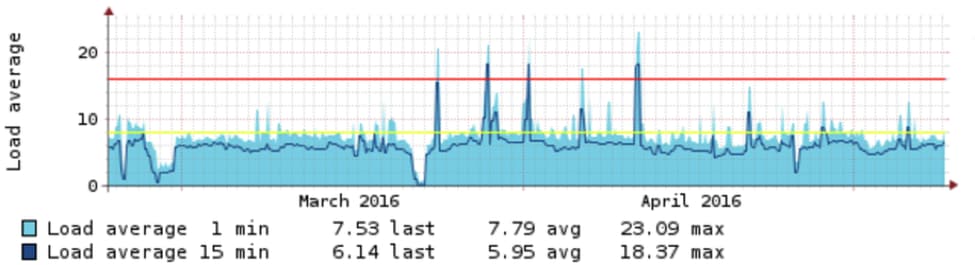
The cpu-load spiking above the red line shows when rebuilding was required
Per-second Mongo cursor pagination queries:
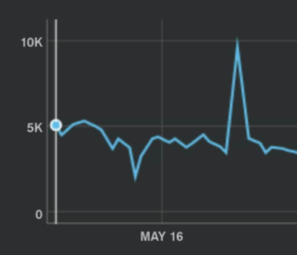
Where are these getmores coming from?
Large number of updates in Mongo
Aperture tracks data as individual objects in the cloud. For example, a file in Box.com is a single unit that can be affected by a variety of possible events that may not be directly on the file itself. This means once we know of the existence of the file, we track changes to it as it updates. This makes Aperture's write load very update-heavy as new objects are far fewer in number than the updates that take place at any point in time. While MongoDB was able to keep up because of its in-place update capabilities, Elasticsearch handled updates by deleting and re-indexing documents that were touched. So, every operation in Mongo resulted in two operations in Elasticsearch, making Elasticsearch do twice the work MongoDB did.
Index Distribution + Oplog
In Elasticsearch, data is stored in indices, divided into shards, that reside on individual Elasticsearch nodes (with copies as required). Each shard is a Lucene index, and large indices have multiple Lucene indexes that handle the data. However, Lucene indices cannot be sharded or combined themselves, and so have to reside on a single node. This means once an Elasticsearch index is created with an appropriate number of shards, those shards cannot be changed. To prevent having one huge index of all customer data, we created indices per customer, with shard counts based on how much data they were expected to have. However, each of these indices was linked to one MongoDB River thread. We had hundreds of MongoDB River threads, and each thread consumed all of the MongoDB oplog and filtered data for the customer it was supposed to index. All of this was done in the Elasticsearch nodes, resulting in a large amount of data egress from MongoDB and a large amount of data crunching and ingress into Elasticsearch – most of which was thrown away, because MongoDB oplog contains data from all namespaces.
Second Attempt: Elasticsearch + Write Layer (or No Free Lunch)
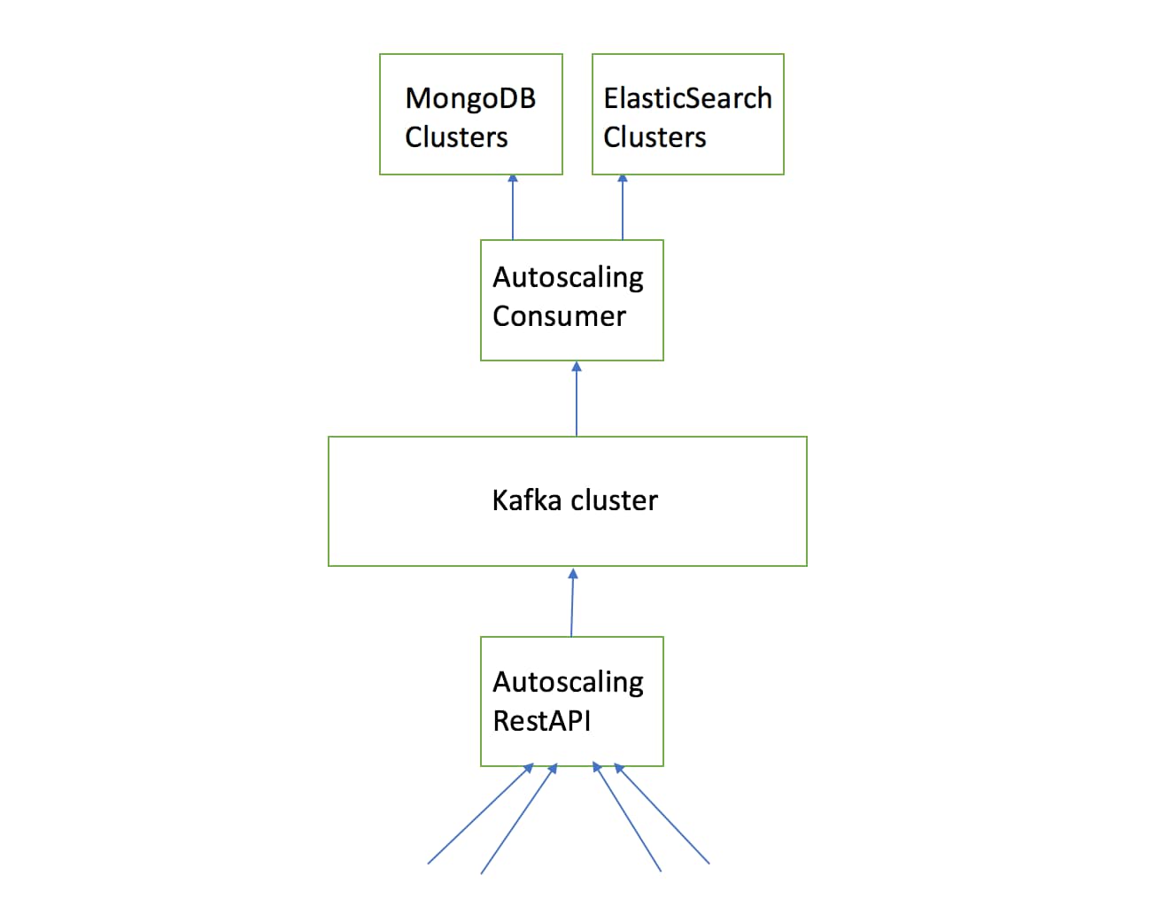
Essentially, we realized that keeping these indices in sync with the persistent data in MongoDB would require a change in our architecture. The solution was to create a database write layer that would pipe the data to both MongoDB and Elasticsearch.
To have such a system, we would need a temporary storage solution for the database writes, and this solution would need to be fault-tolerant and scalable. We decided to use Kafka as the temporary storage solution. Kafka fit in well because of its built-in scalability (using topic partitions) and replication (enabling replication factor). Additionally, Kafka maintains order (within a partition), which provides an option for ordered writes, if required. By committing Kafka offsets only on success, we were able to implement a simple retry by repeating those messages.
This architecture meant our writes were eventually consistent, as the architecture decoupled MongoDB writes from the writers and both databases from each other. However, it also meant we could replay writes that had failed as well as separate Elasticsearch from MongoDB, meaning the databases would be available independent of each other in the event of any reliability issues.
Deploying this solution led to the following results:
Elasticsearch load after:
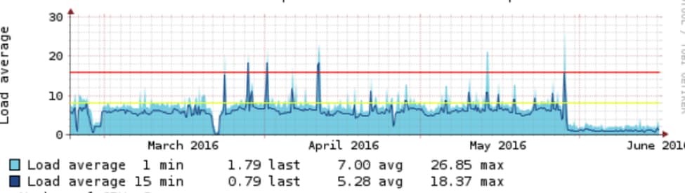
Clear drop from cpu-load of around 10 to 2.
The other half of the MongoDB graph:
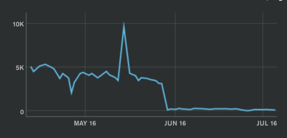
As the graphs indicate, we saw an immediate improvement in the performance of both databases after deployment.
The common write layer led to improved performance on both databases because of lowered connection count and the benefits of using bulk writes instead of single document updates. The lowered CPU and memory pressure allowed us to increase the number of customers per MongoDB replica set by almost an order of magnitude. Additionally, abstracting the database access by using a unified middle layer allowed us to further improve performance by analyzing global queries, adding more granular access control and scale by effortlessly managing the flow of data.
If these are the kinds of technical challenges you like to work on, we would love to hear from you!
Palo Alto Networks engineers help secure our way of life in the digital age by developing cutting-edge innovations for Palo Alto Networks Next-Generation Security Platform. Learn more about career opportunities with Palo Alto Networks Engineering.
Related Blogs
Our library of online content is here to help you learn more, no matter what format you prefer or which topic interests you most.
Subscribe to the Newsletter!
Sign up to receive must-read articles, Playbooks of the Week, new feature announcements, and more.
By submitting this form, you agree to our Terms of Use and acknowledge our Privacy Statement. Please look for a confirmation email from us. If you don't receive it in the next 10 minutes, please check your spam folder.